Load Profiles
Information
Load profiles control how the resource load (for cost resources of the costs) is spread across the duration of the task.
- PLANTA project distinguishes between
- "real" load profiles which cause a percentage distribution of load, and
- "pseudo load profiles the use of which causes a programmed calculation method.
Details
- Which load profile takes effect in the respective task of the respective resource assignment is determined by the Load profile parameter on the resource assignment in the Schedule module.
- Here, the required load profile can be selected via the listbox. If no load profile is selected, the resource load is distributed linearly.
- When you assign a resource to a task, the Default load profile of the resource is applied automatically but can be changed on the resource assignment if necessary.
Notes
- Several real and pseudo load profiles are included in the scope of supply of the PLANTA software.
- You can see them in the Load Profiles module.
- The creation of individual load profiles is currently not supported.
"Real" Load Profiles
Information
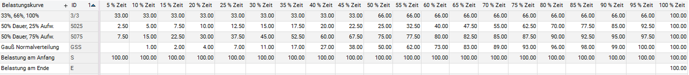
- Real load profiles are defined in 5% steps. When the loads are calculated by the RS procedures, the Remaining duration of the task is divided by 20, and for each of the intervals thus generated, the Remaining effort is multiplied by the difference of the load percentage rates. This results in the distribution of the load.
- The general rule is: duration and effort are predetermined, load is calculated.
Note
- If, e.g., the E and S load profiles are used, it may occur that the load is distributed over more than one day. If the Remaining duration of the task is 60, then 60 / 20 = 3 load records are generated. See examples further below.
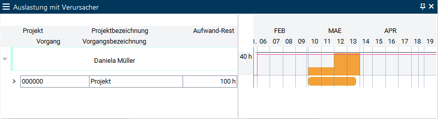
Example utilization diagrams:

Consideration of actual data for real
load profiles
- If the sum of the actual resource load deviates from the planned loads, date scheduling readjusts the remaining loads to the load profile.
Example
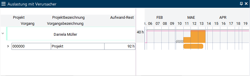
- Starting situation without work reporting
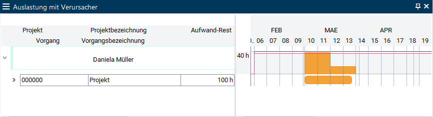
- The Actual effort reported is less than initially planned. The total difference will be loaded on the first day after the work reporting date.
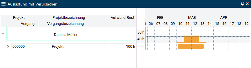
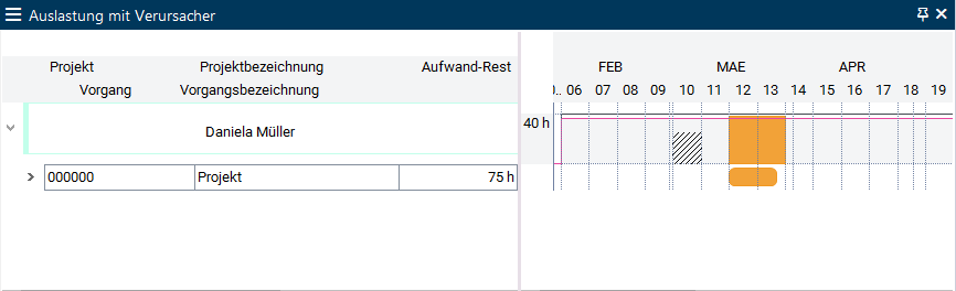
- The Actual effort reported is less than initially planned. in this case, no load will be planned in until the cumulative usage on the original profile is equal to the actual usage so far.
Load Profile E (Load at the End)/Load Profile S (Load at the Start)
Information
- If you use load profile E, loading takes place at the end of the task.
- Load profile S loads at the task start equivalently. The following examples use load profile E.
- One load record is created per 20 days of task duration.
Examples
- Resource R1 is planned for task A with a duration of 10 days and an effort of 100 h.
- The scheduling created a load record with 100h at the end of the task.
- Resource R1 is planned for task B with a duration of 21 days and an effort of 100 h.
- The scheduling creates two load records at the end of the task.
- Load record 1: 4.76 h
- Load record 2: 95.24h
Calculation for task B with Remaining duration = 21 days
- 21 / 20 = 1,05
- 2 load records are created: a load record which corresponds to the entire 20 days and one load record which corresponds to one day.
- The daily load amounts to: 4.76 (=100 / 21)
- The load is distributed in the following order according to the time interval steps.
- Load record 1: 4,76 x 1 = 4,76
- Load record 2: 4,76 x 20 = 95,24
- Resource R1 is planned for task C with a duration of 44 days and an effort of 100 h.
- The scheduling creates three load records at the end of the task:
- Load record 1: 9.09 h
- Load record 2: 45.45 h
- Load record 3: 45.45 h
Calculation for task C with Remaining duration = 44 days
- 44 / 20 = 2,2
- 3 load records are created: 2 load records which correspond to the entire 2 x 20 days and one load record which equates to 4 days.
- The daily load amounts to: 2.27 (=100 / 44)
- The load is distributed in the following order according to the time interval steps.
- Load record 1: 2,27 x 4 = 9,09
- Load record 2: 2,27 x 20 = 45,45
- Load record 3: 2,27 x 20 = 45,45
Note
- The distribution order of the load under load profile S and with the existence of several load records is the exact reverse: large ones first and then the lower ones.
"Pseudo" Load Profiles
Information
From S 39.5.22
- "Pseudo" load profiles (e.g. CAP, MAN, BLD) are based on a programmed calculation method.
- CAP: the load in each period relative to available capacity. The effort of the assigned resource is dominant. In case of scheduling with adherence to float or capacity, the available capacity of the period is scheduled. The duration is calculated.
- BLD: Basic Load. It is used to plan the basic load projects along with the Max. load/day parameter. Without Max. load/day it takes effect as a linear load profile.
- MAN: Manual load per period
- NEW PM_DAY, PM_MONTH, PM_WEEK, PM_QUART, PM_YEAR: Manual persistent load per time grid. For a detailed description, see here.
Up to S 39.5.22
"Pseudo" load profiles (e.g. CAP, MAN, BLD) are based on a programmed calculation method.
- CAP: the load in each period relative to available capacity. The effort of the assigned resource is dominant. In case of scheduling with adherence to float or capacity, the available capacity of the period is scheduled. The duration is calculated.
- BLD: Basic Load. It is used to plan the basic load projects along with the Max. load/day parameter. Without Max. load/day it takes effect as a linear load profile.
- MAN: Manual load per period
CAP Load Profile
Information on the CAP load profile can be found
here...
MAN Load Profile
Information on the MAN load profile can be found
here...
BLD (Basic Load) load profile
Information on the BLD load profile can be found
here...
No Load Profile: Linear load distribution
Information
- In linear load distribution, the Remaining effort is distributed linearly to the Remaining duration of the task.
- Overloads are not adjusted but only identified.
- The linear load distribution is carried out if no Load profile has been selected for a task resource.
Example
- Remaining duration = 10 days.
- Remaining effort = 100 hours
- Hence, load 100/10=10 hours per day
- If the resource has an availability of 8 hours per day, 2 hours of overload are shown on each day.
Load Profiles with Time Grid: WEEK, MONTH , QUARTER, YEAR
Information
- If you use the WEEK, MONTH, QUARTER or YEAR load profiles, only one load record is created per week, month, quarter, or year.
- The objective of the use of these load profiles is an acceleration of long-term analysis (e.g. utilization diagrams) by the reduction of load records.
Notes
- When you use the WEEK, MONTH, QUARTER, and YEAR load profiles,
Details on remaining loads
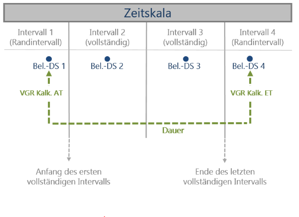
- In the first step, the scheduling calculates the load records exactly to the day (in the background).
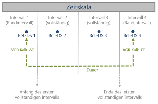
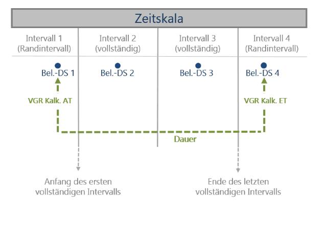
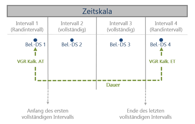
- In the next step, the load records are summarized by the scheduling to the following points in time:
- for complete intervals to the middle of the respective interval
- WEEK: load only on the Wednesday of each week
- MONTH: load only on the 15th of each month
- QUARTER: load only on the 15th of the middle month
- YEAR: load on July 15th of a year
- Please note that in scheduling the 15th of a month is not treated as a real date but only as an interval marker. I.e. in case the 15th is a non-working day, loading is executed on that day anyway.
- for the margin intervals it is loaded on the TAR Calc. start and TAR Calc. end. This means:
- The date of the last planned load record equates to the TAR _Calc. start.
- The date of the last planned load record equates to the TAR _Calc. end.
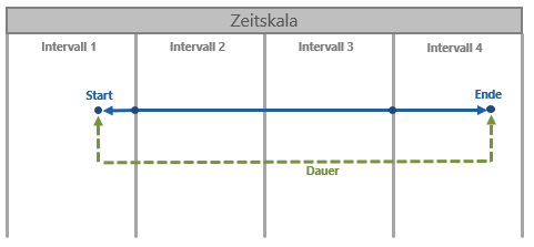
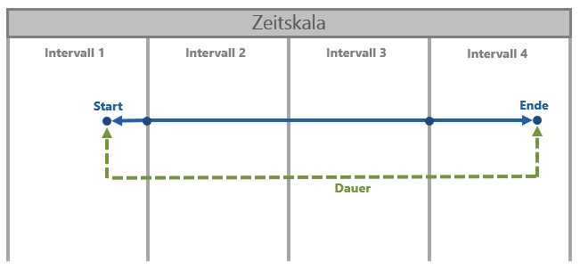
Schematic display
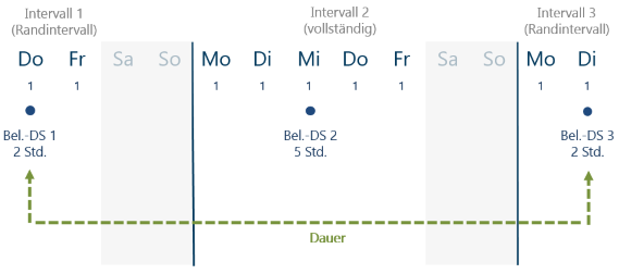
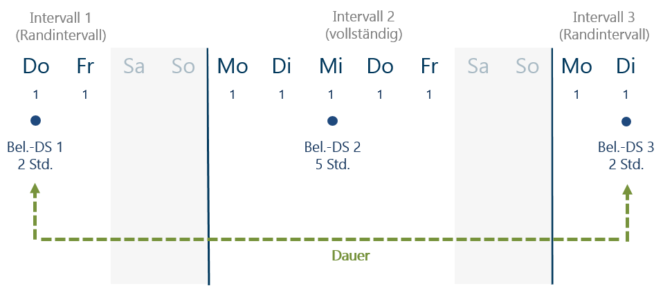
Application example:
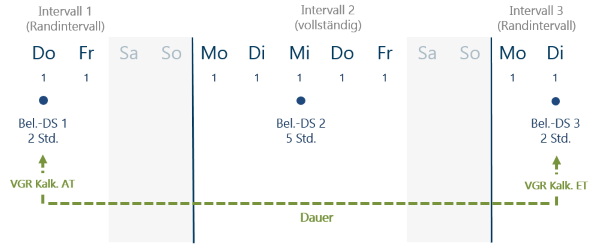
- A task with a duration of 9 days and a resource assignment with WEEK load profile and Remaining effort = 9 h begins on a Thursday and ends a week later on a Tuesday.
- In the first step, the scheduling distributes the 9 hours evenly among the 9 days, resulting in a load of 1 hour per working day.
- In the second step, scheduling summarizes the distributed hours to one load record per interval.
- The 1st summarized load record contains the data from Thu Fri and has TAR Calc. start (=Thursday of the first week) as a date.
- The 2nd summarized load record contains the data from Mon Fri and has the Wednesday of the second week as a date
- The 3rd summarized load record contains the data from Mon Tue and has TAR Calc. end (= Tuesday of the 3rd week).
- As a result of summarization, inaccuracies may occur in the summarized values. It is recommended that replanning is carried out cyclically.
- The grid for the analyses (e.g. for utilization diagram) should be equal to, or greater than the summarization time grid; e.g. if the display is shown to the day for a summary on an annual time grid, all loads would appear on 07/15.
Details on actual loads
- Since working time recording is done per day, the actual records exist day-wise, independent of the selected grid.
Manual Load Profiles with Time Grid (PM_*) New from S 39.5.22
Load profiles for manual distribution of effort in time intervals
- PM_DAY
- PM_MONTH
- PM_WEEK
- PM_QUART
- PM_YEAR
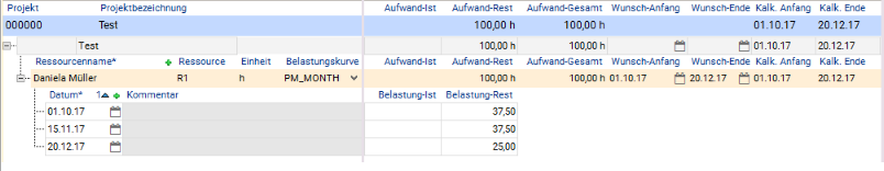
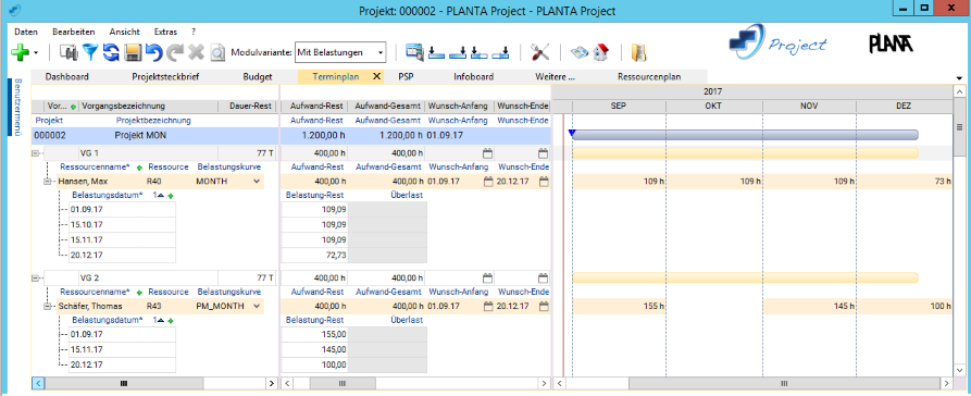
Application example: Other than regular load profiles, manual load profiles with time grid allow you to, e.g., interrupt the planning of a resource in a task.
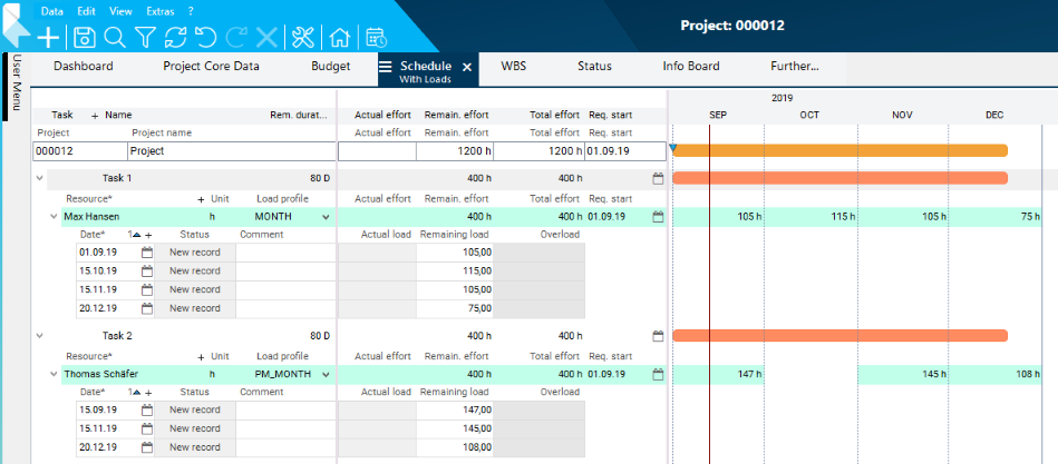
Procedure
- When using the PM_interval load profiles, you can choose between two procedures.
- Procedure 1
- Define effort and requested dates on the resource assignment (for this purpose, see the note further below) and calculate the schedule. As a result, this effort is automatically allocated according to the equivalent time grid load profile (PM_WEEK according to WEEK, PM_MONTH according to MONTH, PM_QUART according to QUARTER and PM_YEAR according to YEAR), however, only initially. Afterwards, load profiles can be edited manually. Load profiles remain unchanged after each further scheduling. Only the remaining load is recalculated (e.g. actual effort subtracted in opposite to MAN load profile) and summarized to the resource assignment.
- This procedure can e.g. be used as an input assistance.
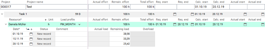
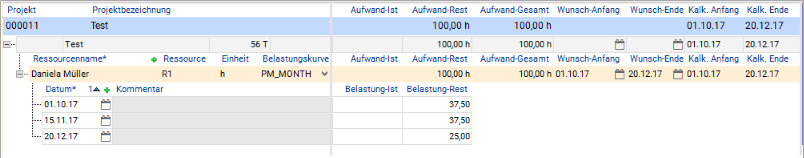
- Procedure 2
- Initially you manually create load records in accordance with the selected interval. In this procedure, the manually created records are not changed from the first scheduling on. The data is only summarized upwards. In each further scheduling, the load records also remain unchanged. Only the remaining load is recalculated (e.g. actual effort subtracted in opposite to MAN load profile) and summarized to the resource assignment.
- This procedure is recommended by PLANTA.
Notes
- For a task that possesses a resource assignment with PM_interval load profile, the following parameters are set automatically
Attention
Due to these limitations and in order to guarantee the correct functionality of the PM_interval load profile, you are recommended to use requested dates instead of remaining duration in both cases mentioned above.
Particularities of Manual Load Profiles with Time Grid
Notes
- The general information and details for the intervals and the distribution of load records per interval which are described in the "Load Profiles with Time Grid: WEEK, MONTH, QUARTER, YEAR" section also apply to the manual time grid load profiles
- In the following, only particularities of the manual time grid load profiles are listed.
Details
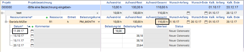
- Since only one Remaining record (plan record) is allowed per interval, every further remaining record recorded in the same interval is consolidated with the record which was created first, i.e. the load is added to that of the first record.
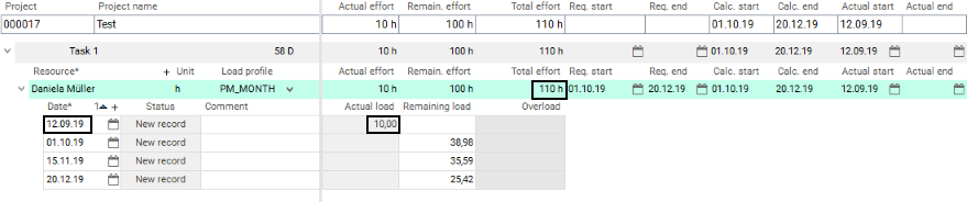
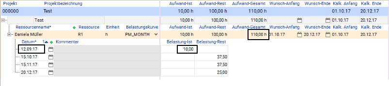
Details on work reporting
- If the entire planned effort is reported to an interval as actual effort, the remaining effort is set to 0, the respective remaining record (planning record), however, is retained.
- If more working hours are reported in an interval than planned, the remaining effort is set to 0 as well, but the total effort is increased as those hours are not subtracted from the planned effort of other intervals.
- If hours are reported in an unplanned interval, the total effort is increased since the hours cannot be subtracted from the effort planned in other intervals.
Example
Attention
- When planning with PM interval load profiles > PM_DAY, there may be differences in overloads in DT472 and DT468 to be considered. If there are, e.g., overloads on period level, they may be compensated in the week or month planning data and therefore not be specified in DT472.
Reason: The loads are linearized to interval granularity since the saving only contains the total effort, etc., over the respective period, and not the number of affected working days. Overloads are therefore only specified on interval granularity. Overload only occurs in a load record if the remaining effort exceeds the availability in the entire period in question.
Differences between MAN and PM_DAY
| MAN |
|
PM_DAY |
| There is only one record per day (period): remaining or actual. If actual hours are recorded for a day, the entire remainder for the day in question is deleted in date scheduling. |
≠ |
There is one remaining record and possibly several actual records per day (period). The remaining record is always retained, the actual records are added. |
| Work reportings do not change the planned hours. |
≠ |
The reported hours are subtracted from the planned hours. If a new load record is added to a defined interval, the remaining effort is increased respectively. |
| Planning hours of the MAN load profile that are earlier in time than the first work reporting are deleted and not distributed to future loadings. |
≠ |
Planning hours of the PM_DAY load profile that are earlier in time than the first work reporting are deleted and not distributed to future loadings. |
| Reporting of hours worked with a different value than planned do not affect the other load records. |
= |
Reporting of hours worked with a different value than planned do not affect the other load records. |
| Hours planned for task resources using the MAN load profile are not shifted by the scheduling. |
= |
Planning hours for task resources using the PM_DAY load profile are not shifted by the scheduling. |
 .
. 
